Two policy gradients, one blind spot
This distinction appears across reinforcement learning. PPO and GRPO use the score-function route [1], [2], [3]. SAC and differentiable simulation use pathwise derivatives, although they obtain those derivatives from different places [4], [5]. The names will make more sense after we solve one small robot problem. First, here is the whole setup in one picture: the input stays fixed, but a stochastic policy can sample different actions.
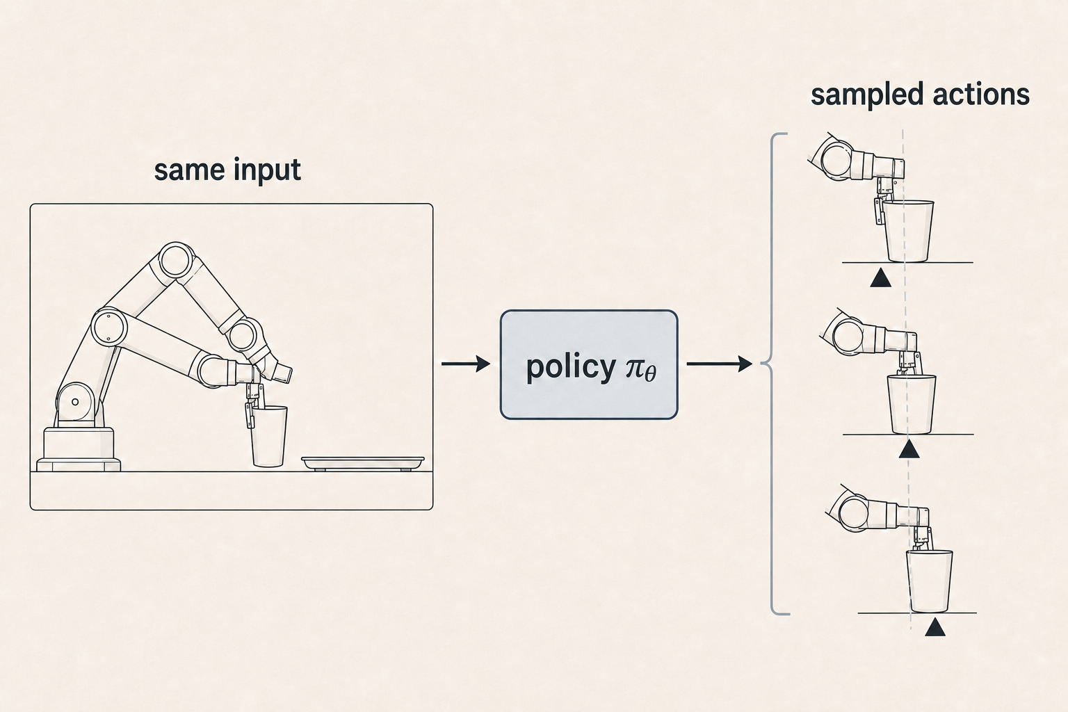
Start with one noisy robot action
Imagine that the robot repeats the same reach many times. The camera image, instruction, cup, and all but one joint stay fixed. The only number we record is where the gripper closes along the horizontal axis. Call this position , measured in centimetres from the cup’s centre.
We model the action as
Here is the mean position chosen by policy parameters , is the amount of exploration noise, and is one draw from a standard normal distribution. In plain language: the policy aims at , but each attempt lands a little to the left or right.
The robot receives one point if the gripper closes inside the success interval , and zero otherwise:
The symbol is an indicator: it equals when the condition is true and when it is false. Throughout the post, cm and cm. This reward has no gentle slope: crossing either edge changes the reward instantly from to , or from to .
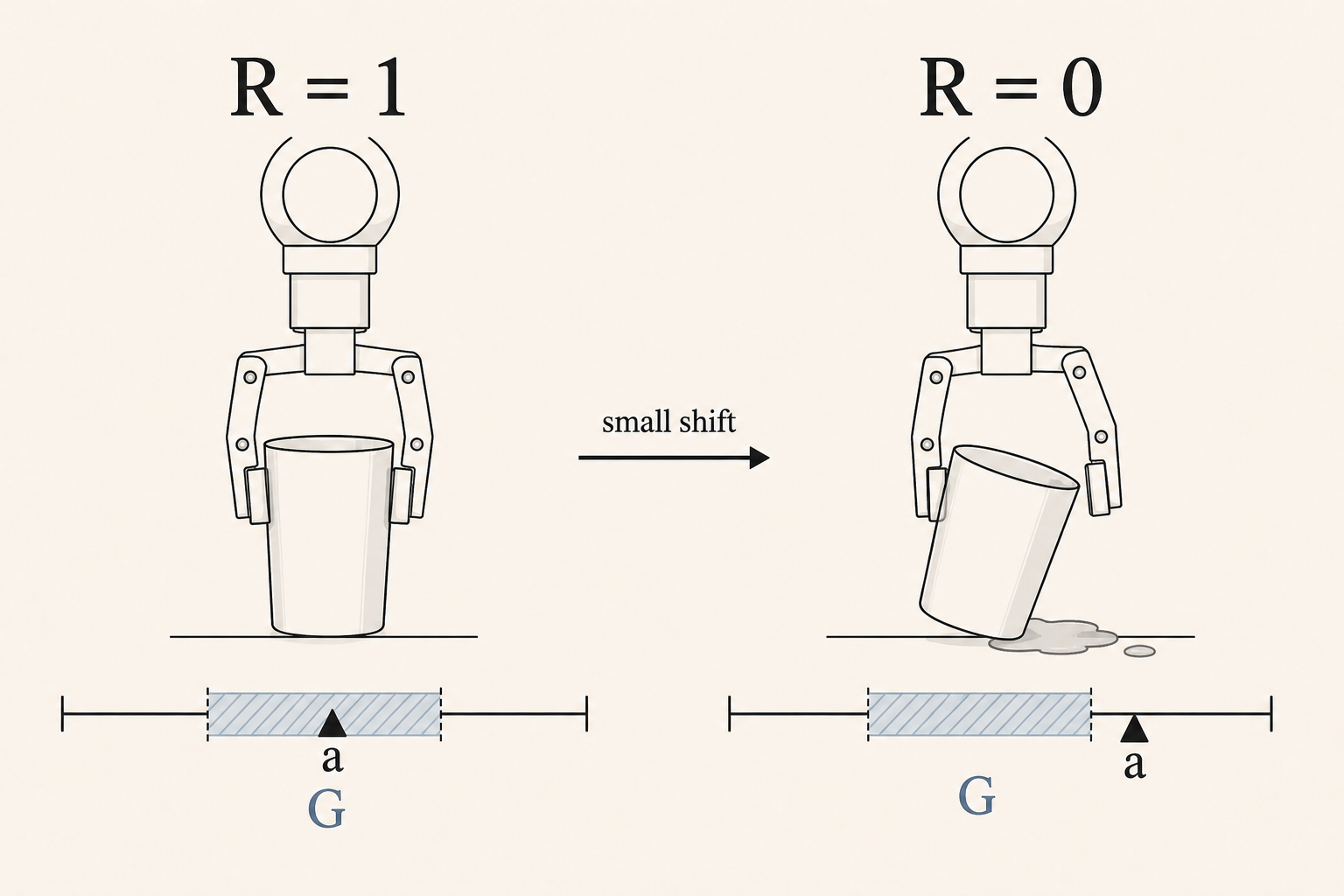
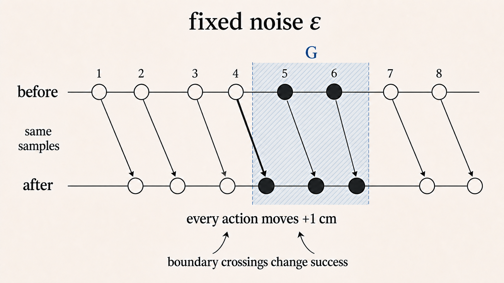
The second figure deliberately tells the same story twice. The robot drawings show the physical consequence; the strips below them show the mathematical abstraction. The next diagram adds the policy’s full action distribution on top of that line.
![A Gaussian policy density centred at μ = −3 cm, with the area under the curve inside the hatched success interval G = [−2, 2] cm shaded as the success probability J(μ).](/assets/posts/robot-two-gradients-one-flow/policy-density.png)
A policy update moves probability
Before deriving either gradient estimator, we need a precise description of what learning changes. Let run continuously from to as the policy moves from its old parameters to its new ones: and . This is not the robot’s physical time . The index moves the robot through one rollout; moves the policy through one update.In the one-action example, we can simply set . Increasing then means sliding the Gaussian policy to the right.
A rollout is one complete sequence of states and actions. Let be the probability density that the current policy and environment assign to that rollout, and let be its total reward. The objective is the expected reward:
Equation (1) says: consider every possible rollout, multiply its reward by its probability, and add the results. The integration variable means that the integral ranges over all possible rollouts. For a fixed task, the scoring rule stays the same. The policy update changes , so it changes which rollouts are likely.
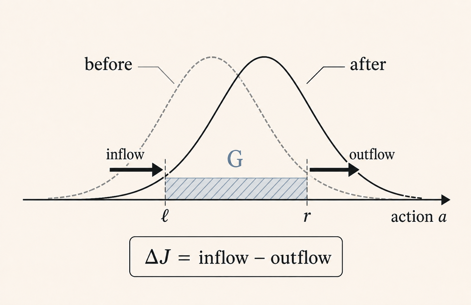
We can describe this change as a flow of probability. Let be a velocity field: it tells us the direction and speed at which probability near rollout moves as increases. Conservation of probability gives the continuity equation:
The first term, , is the rate at which the density changes at a fixed location. The second term measures net probability flowing out of that location: is the probability flux, is its divergence, and the minus sign says that net outflow lowers the local density. In short, density changes because probability flows in or out; probability is not created or destroyed.
The one-dimensional robot example makes (2) easy to check. Set and shift the Gaussian mean to the right. Every sampled action moves right at unit speed, so . The equation becomes : changing the mean has the same effect as translating the whole density in the opposite coordinate direction.
Probability in a region falls not because probability was destroyed, but because it went somewhere else.
View one: keep the outcomes fixed
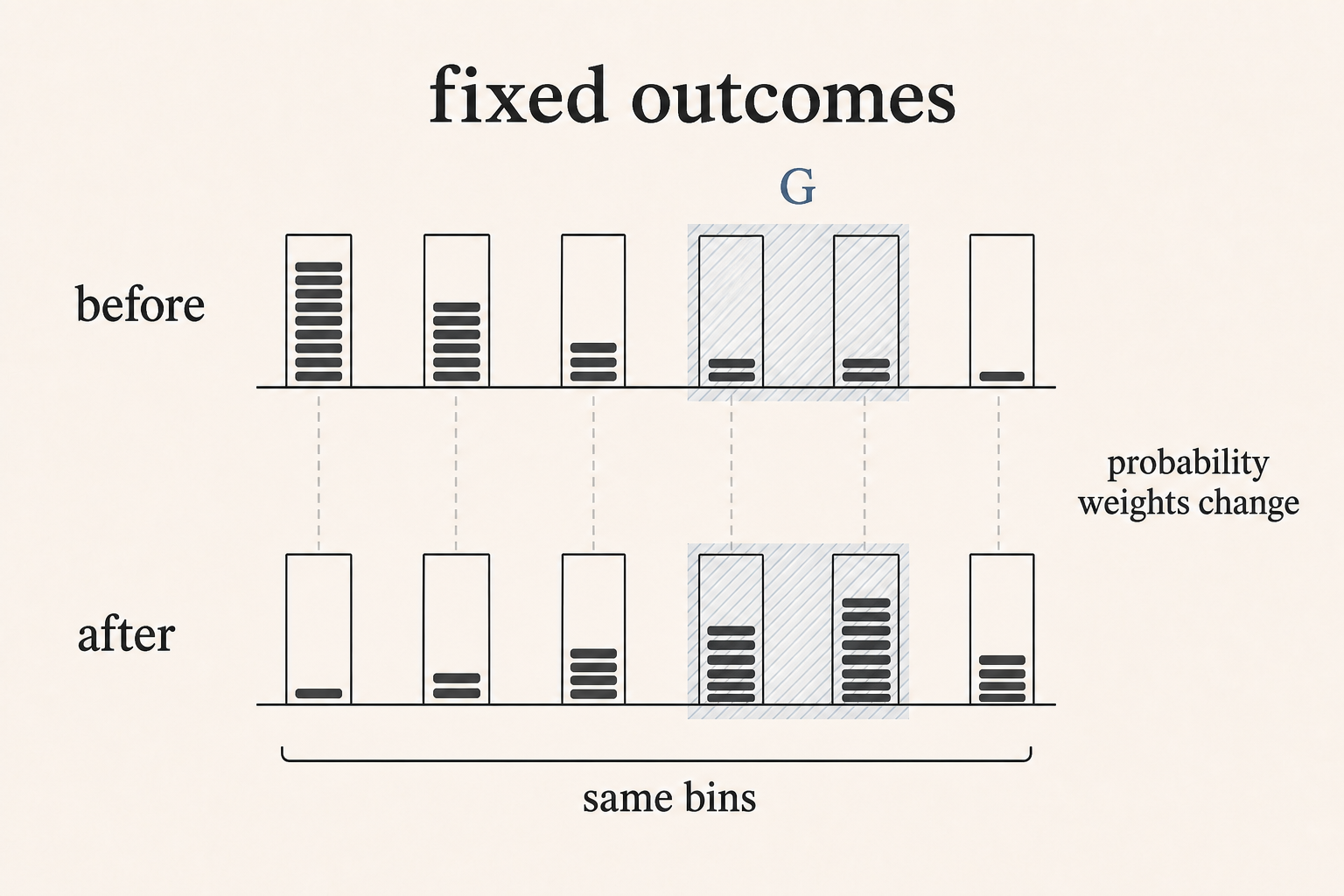
The first view keeps each possible rollout fixed and asks how its probability changes. Differentiate (1) with respect to . Because the task reward does not depend on the policy update, the derivative acts only on :
The last expression is the score-function, or likelihood-ratio, gradient. The reward says how good the sampled rollout was. The score says how quickly the update changes that rollout’s relative probability. Their product is the rollout’s contribution to the gradient, and the expectation averages that contribution over sampled rollouts.
Why can this estimator work with a black-box environment? The probability of a rollout factors into the initial-state distribution , the policy , and the environment dynamics :
The product on the left assigns a probability to the whole rollout. After taking the logarithm, that product becomes a sum. If the environment does not itself depend on , the derivatives of and are zero, so only derivatives of the policy remain on the right. We need sampled states, actions, and rewards, plus from the policy network. We do not need derivatives of the environment or reward. This is the key idea behind REINFORCE [7] and the policy gradient theorem [8].
This route is tolerant of black boxes, but it is not assumption-free. Moving the derivative through the integral must be valid, and the set of possible rollouts—the support of —must behave regularly. If the support itself changes shape with , the usual formula needs extra care [9].
View two: keep the randomness fixed
The second view matches an outcome under the old policy with an outcome under the new one. Write for a random draw from a fixed noise distribution, and write for the rollout produced by passing that draw through the policy and environment. In the robot example, this is simply .
The important step is to give the old and new policies the same . Think of as a numbered lottery ticket. If both policies receive the same ticket, we can say how that particular sampled outcome moved. If they receive independent tickets, we can compare two distributions, but we cannot match one old sample to one new sample.
With shared noise, is the velocity of the sampled rollout. If the reward is differentiable along this path, the chain rule gives the pathwise gradient:
The vector is the local reward slope: it points toward nearby rollouts with higher reward. The vector says how the sampled rollout moves as the policy changes. Their dot product measures how quickly the reward changes along that motion, and the expectation averages over noise draws.
For a multi-step rollout, we can write for the policy and for the environment. Here maps a state and policy noise to an action; maps the current state, action, and environment noise to the next state. Once every and is held fixed, the rollout becomes an ordinary computation graph, , and backpropagation can differentiate it. Stochastic computation graphs formalize how score-function and pathwise estimators can be mixed at different random nodes [10].
Integration by parts connects the two views
The two formulas look unrelated: (3) differentiates probability, while (4) differentiates reward. The continuity equation shows that they describe the same flow. Substitute into the score-function derivation, then use integration by parts to move the derivative from the probability flux onto the reward:
The left expression is the score-function view: keep locations fixed and watch their probability weights change. The middle expression replaces that weight change with probability flow. The right expression is the pathwise view: follow the moving probability and measure the reward slope along its path. Integration by parts is the operation that moves the derivative from to .
claim 1 (two views of one gradient).
This transport interpretation of pathwise derivatives is developed by Jankowiak and Obermeyer [6]. Parmas and Sugiyama give a unified treatment of likelihood-ratio and reparameterization gradients as estimators of the same probability movement [11].
Three caveats are important. First, equal expectations do not imply equal finite-sample variance. Second, the velocity field is not unique, so different pathwise estimators can have the same mean. Third, claim 1 assumes that the ordinary reward gradient exists. Our hard reward breaks that last assumption.
Where common algorithms fit
We can now sort familiar algorithms by one practical question: what derivative can the algorithm obtain outside the policy itself? The “view” column follows from that requirement.
| family | view | derivative needed outside the policy | hard |
|---|---|---|---|
| REINFORCE, PPO, GRPO [1], [2], [7] | fixed outcomes | none; only sampled returns | unbiased, but can be noisy |
| DDPG, TD3, SAC [4], [12], [13] | fixed noise | from a learned critic | depends on the critic’s learned smoothness |
| SVG(1), SVG() [14] | fixed noise | derivatives through a learned dynamics model | depends on the learned model and reward |
| differentiable simulation [5] | fixed noise | dynamics and reward derivatives from the simulator | naive autodiff returns zero in this example |
| Gumbel-Softmax, straight-through [15] | fixed noise | a differentiable relaxation of a discrete choice | produces a biased surrogate gradient |
The actor-critic row is easy to misunderstand. DDPG and SAC do not differentiate the real environment. They differentiate a learned critic with respect to the action. The smoothness requirement therefore falls on a neural network the algorithm controls, not directly on the world’s reward or dynamics. By contrast, methods that backpropagate through a learned dynamics model or a differentiable simulator need a longer differentiable path. Evolution strategies and random search sit outside both columns: they estimate changes in performance without forming at all [16], [17].
One boundary is enough to fool autodiff
Return to the robot’s actual reward and set the update coordinate equal to the policy mean . The objective is now simply the probability that a Gaussian action lands between and . Let denote the standard normal cumulative distribution function and its probability density. Then both the objective and its exact derivative have closed forms:
The formula for subtracts the Gaussian probability to the left of from the probability to the left of , leaving exactly the probability inside the success interval. The derivative has an equally concrete meaning: is probability density entering through the left edge as the policy moves right, while is density leaving through the right edge. Their difference is inflow minus outflow.
The same conclusion follows directly from the continuity equation. Integrating (2) over gives
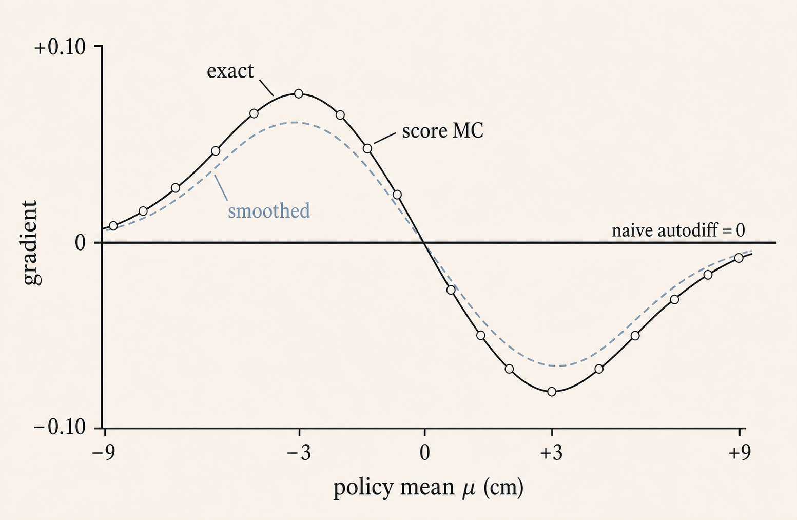
The two terms are the probability flux through the interval’s left and right edges. In our example , so the gradient is , matching the formula above and figure 4.This boundary is not the boundary term at infinity in claim 1. It appears because we integrate over the finite success interval .
The score-function view has no problem with this boundary because it never differentiates the reward. For one sampled action, its gradient estimate is
The reward says whether the sample succeeded. The factor is the derivative of the Gaussian log-probability with respect to its mean. Averaging these products gives an unbiased estimate: over repeated sample sets, its mean equals the exact gradient.
Now apply ordinary autodiff through the same sampled action. The chain rule produces
The action moves one-for-one with , which explains . But the indicator reward is flat everywhere except at its two edges, so ordinary autodiff sees for every sample that does not land exactly on an edge. A continuous distribution hits either exact edge with probability zero. Therefore the estimator is not merely noisy: it returns exactly zero for every practical sample set, at every .
Why is the true gradient nonzero? Because success improves when probability crosses the boundary, not because reward has a local slope inside either flat region. In figure 6, all particles shift by the same amount. The change in success count comes entirely from particles crossing into or out of . Pointwise autodiff examines the neighborhood around each sampled particle, so it misses a contribution concentrated exactly at the edges.
In generalized-function notation, the missing derivative is
where the Dirac delta represents a unit contribution concentrated at one point. Substituting this generalized derivative into (4) with recovers . So the pathwise identity is not mathematically wrong. The problem is that ordinary autodiff differentiates the program’s pointwise operations and does not automatically recover this boundary contribution.
| μ (cm) | J(μ) | exact ∂J/∂μ | score, MC mean | ± s.e. | naive pathwise | smoothed, β = 2 |
|---|---|---|---|---|---|---|
| −9.0 | 0.0097 | 0.00858 | 0.00836 | 0.00027 | 0 | 0.01046 |
| −6.0 | 0.0874 | 0.05087 | 0.05088 | 0.00052 | 0 | 0.05169 |
| −3.0 | 0.3217 | 0.09264 | 0.09208 | 0.00046 | 0 | 0.08558 |
| 0.0 | 0.4950 | 0.00000 | 0.00031 | 0.00025 | 0 | 0.00092 |
| 3.0 | 0.3217 | −0.09264 | −0.09178 | 0.00046 | 0 | −0.08516 |
| 9.0 | 0.0097 | −0.00858 | −0.00874 | 0.00026 | 0 | −0.01016 |
For example, when cm, the robot succeeds about of the time and the exact gradient is . The score-function Monte Carlo mean is , close to the exact answer. Naive pathwise autodiff still reports , while the smoothed reward reports —a useful direction, but a biased value for the original objective.
A common workaround is to replace each hard step with a smooth sigmoid:
Here is the logistic sigmoid, and controls how sharp the two softened edges are. This surrogate reward has nonzero slopes near and , so autodiff can see a pathwise signal. But it is a different objective. At , the resulting gradient is about too small at and about too large at ; the bias even changes sign. Increasing makes the surrogate closer to the hard reward, but it also concentrates the useful gradient into narrower regions near the edges, which tends to increase variance.
The exact objective, exact derivative, score-function estimate, and variance calculation fit in a few lines of dependency-free Python. The code below makes the numerical claims reproducible.1
import math

SIGMA, L, R = 3.0, -2.0, 2.0

def phi(x): return math.exp(-0.5 * x * x) / math.sqrt(2.0 * math.pi)
def Phi(x): return 0.5 * (1.0 + math.erf(x / math.sqrt(2.0)))

def J(mu):
    """Success probability in closed form."""
    return Phi((R - mu) / SIGMA) - Phi((L - mu) / SIGMA)

def dJ(mu):
    """Its exact derivative: density at the left edge minus density at the right."""
    return (phi((L - mu) / SIGMA) - phi((R - mu) / SIGMA)) / SIGMA

def score(mu, n, rng):
    """Unbiased at every mu; needs only sampled successes and failures."""
    xs = [mu + SIGMA * rng.gauss(0.0, 1.0) for _ in range(n)]
    return sum((1.0 if L <= a <= R else 0.0) * (a - mu) / SIGMA**2 for a in xs) / n

def score_sd(mu):
    """Exact standard deviation of one score sample, via int u^2 phi(u) du."""
    ul, ur = (L - mu) / SIGMA, (R - mu) / SIGMA
    m2 = (ul * phi(ul) - ur * phi(ur) + Phi(ur) - Phi(ul)) / SIGMA**2
    return math.sqrt(m2 - dJ(mu) ** 2)

# The naive pathwise estimator is a function that sums zeros, so it is not written here:
# dR/da is 0 wherever it exists, and the mean of n zeros is 0 for every n.
What each view costs
The score-function estimator can see a hard boundary, but rare successes make it noisy. If one sample has standard deviation and the true gradient has magnitude , then the number of independent samples needed for a standard error equal to of is approximately
This equation comes from the usual standard error . As the policy mean moves away from the cup, success becomes rare, becomes small relative to the estimator’s noise, and the required sample count grows rapidly:
| μ (cm) | J(μ) | exact ∂J/∂μ | s.d. of one sample | ratio to gradient | samples for 10% error |
|---|---|---|---|---|---|
| −3.0 | 3.2e−01 | 9.26e−02 | 0.151 | 1.6 | 265 |
| −6.0 | 8.7e−02 | 5.09e−02 | 0.168 | 3.3 | 1084 |
| −9.0 | 9.7e−03 | 8.58e−03 | 0.087 | 10.2 | 10331 |
| −12.0 | 4.3e−04 | 5.12e−04 | 0.025 | 48.5 | 234806 |
| −15.0 | 7.3e−06 | 1.11e−05 | 0.004 | 369.6 | 13657178 |
The two views therefore fail in opposite ways on the same task:
- The score-function view sees the correct boundary flux without differentiating the reward, but it needs many samples when successes are rare.
- The pathwise view often provides a low-variance local signal when the computation is smooth, but ordinary autodiff sees no signal at all from this hard boundary.
This does not contradict claim 1. The theorem equates the ideal expectations under its regularity assumptions; it does not promise that every finite-sample implementation is useful, or that ordinary autodiff will construct the generalized derivative of a discontinuity.
Read table 1 with that tradeoff in mind. PPO and GRPO can learn from a reward, but may pay heavily in samples. A differentiable simulator given the same raw indicator reward can return zero because the gradient it computes contains no boundary term.One practical compromise is to use an accurate simulator for the forward pass and a smoothed surrogate for the backward pass [19].
The main lesson is simple: a policy gradient measures how probability moves between outcomes. You can estimate that movement by watching probability weights change or by following samples through the computation. Hard reward boundaries make the choice visible: the true gradient lives in probability crossing the boundary, and an estimator is useful only if it can see that crossing.
Footnotes
references
cite
Found this useful or inspiring? Consider citing it — and follow along on X.
@article{feng2026robottwo,
  title   = {Two policy gradients, one blind spot},
  author  = {Feng, Aosong},
  journal = {asfeng.dev},
  year    = {2026},
  month   = {Aug},
  url     = {https://asfeng.dev/blog/robot-two-gradients-one-flow/}
}
© 2026 Aosong Feng · text licensed CC BY 4.0 — quote and reuse with attribution.